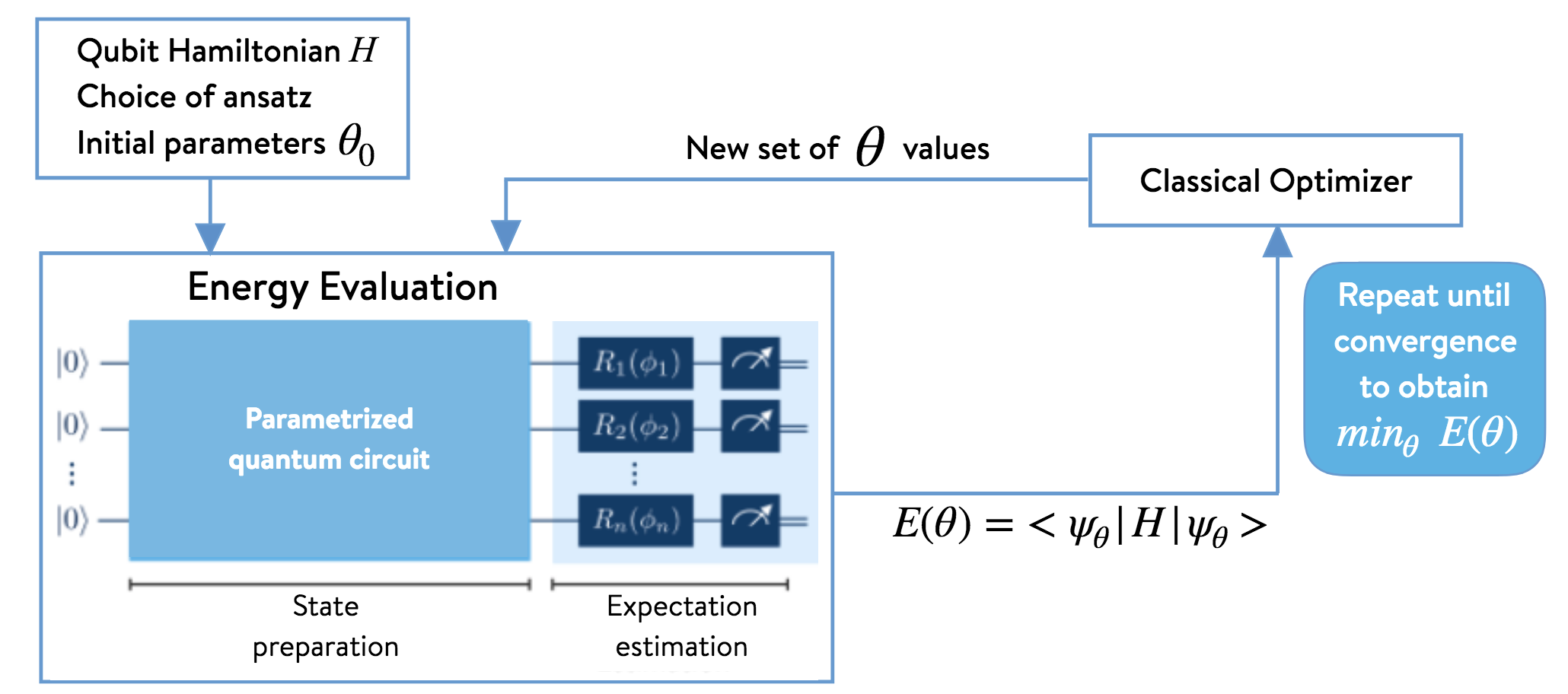
The Variational Quantum Eigensolver (VQE) is an algorithm developed for quantum chemistry applications to run on quantum computers. In our previous tutorial on Introduction to PennyLane, we explored the concept of differentiable programming and setting up variational circuits. VQE is used to find a wave function ansatz(an educated guess) of a molecule like Hydrogen or Lithium Hydride and estimate the expectation value of its Hamiltonian while a classical optimizer is used to adjust the quantum circuit parameters in order to find the molecule’s ground state energy.

We will be using the PennyLane library to find the ground state energy of the hydrogen molecule. We will import the qchem library which is the quantum chemistry library of PennyLane. We will follow three steps in the tutorial:

1. Define the quantum circuit to prepare the ansatz or trial wavefunction
2. Calculate the expectation value of the observable quantity of the hamiltonian
3. Optimize circuit parameters to compute molecular properties

import pennylane as qml
from pennylane import qchem
from pennylane import numpy as np

Step One : Finding the Electronic Hamiltonian

The electronic hamiltonian depends on three properties: the geometry and charge of the molecule, and the spin multiplicity of the electronic configuration.

geometry = 'h2.xyz'

The charge specifies the number of electrons that have been added(for molecules with electron affinity) or removed(ionized) from the neutral molecule. Since we are considering the hydrogen molecule, we will take the charge to be 0.

charge = 0

The multiplicity parameter(or how the electrons occupy the molecular orbitals) is related to the number of unpaired electrons in the Hartree-Fock state. For the neutral hydrogen molecule, the multiplicity is 1.

multiplicity = 1

We also need to specify the basis set used to approximate atomic orbitals. This is typically achieved by using a linear combination of Gaussian functions. We will use the minimal basis STO-3g which is a set of 3 Gaussian function.

basis_set = 'sto-3g'

The molecule’s Hamiltonian is computed in the Pauli basis which is the most common type of basis used for performing such computations. With PennyLane, the hamiltonian can be computed in the Pauli basis by calling the function molecular_hamiltonian(). The first input to the function is a string which is the name of the molecule.

name = 'h2'

The number of active electrons, active orbitals is also specified as well as the fermionic-to-qubit mapping, which can be either Jordan-Wigner (jordan_wigner) or Bravyi-Kitaev (bravyi_kitaev). The outputs of the function are the qubit Hamiltonian of the molecule.

h, qubits = qchem.molecular_hamiltonian(
    name,
    geometry,
    charge=charge,
    mult=multiplicity,
    basis=basis_set,
    active_electrons=2,
    active_orbitals=2,
    mapping='jordan_wigner'
)

print('Number of qubits = ', qubits)
print('Hamiltonian is ', h)

Step Two : Implement the VQE Algorithm

The ExpvalCost class is used to implement the VQE algorithm. First we will define our backend simulator.

dev = qml.device('default.qubit', wires=qubits)

Step Three : Create the quantum circuit to prepare the ground state of the input Hamiltonian

We will develop a circuit which encode the ground state wave function of the hydrogen molecule described with a minimal basis set. For h2, the qubit register is initialized to |1100⟩ as it encodes the Hartree-Fock state of the hydrogen molecule described with a minimal basis. The reason why we chose this circuit is because it is easy to optimize and describes the wavefunction with minimal basis set.

def circuit(params, wires):
    qml.BasisState(np.array([1, 1, 0, 0], requires_grad=False), wires=wires)
    for i in wires:
        qml.Rot(*params[i], wires=i)
    qml.CNOT(wires=[2, 3])
    qml.CNOT(wires=[2, 0])
    qml.CNOT(wires=[3, 1])

Step Four : Call the Cost Function for Optimizing the Circuit

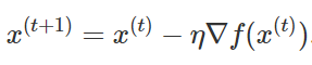
A gradient descent optimizer is used to optimize the cost function. The gradient descent optimizer computes the new values via the following equation. We are keeping the step size as 0.4 which will allow the algorithm to converge fast.

cost_function = qml.ExpvalCost(circuit, h, dev)
opt = qml.GradientDescentOptimizer(stepsize=0.4)
np.random.seed(0)
params = np.random.normal(0, np.pi, (qubits, 3))

print(params)

Step Five : Iterate the Optimization over 200x until Convergence

We will iterate 200 times so to reach the convergence tolerance.

max_iterations = 200
conv_tol = 1e-06


for n in range(max_iterations):
    params, prev_energy = opt.step_and_cost(cost_fn, params)
    energy = cost_fn(params)
    conv = np.abs(energy - prev_energy)

    if n % 20 == 0:
        print('Iteration = {:},  Energy = {:.8f} Ha'.format(n, energy))

    if conv <= conv_tol:
        break

print()
print('Final value of the ground-state energy = {:.8f} Ha'.format(energy))

The output is:

Final value of the ground-state energy = -1.13615709 Ha

The calculated ground state energy is close to the exact ground state energy of 1.1361894 Hartree (Ha).